Mathematical Derivation
Recall the objective is to compute, for all \(i=1,\ldots m\),
\[ \begin{align}\begin{aligned}\sum_{j=1}^m q_j\text{sinc}(\mathbf{a_i}-\mathbf{k_j})\\\sum_{j=1}^m q_j\text{sinc}^2(\mathbf{a_i}-\mathbf{k_j})\end{aligned}\end{align} \]
We will exploit the fact that the the FINUFFT library quickly computes expressions of the form
\[\sum_{j=1}^m f(x_j)e^{\pm i x_j k_r} \qquad \mbox{ for all } r=1,\ldots,n\]
much faster than the naive \(O(nm)\) time, where the points \(x_j\) and \(k_r\) may be arbitrarily spaced.
Conventions
\[ \begin{align}\begin{aligned}\mathcal{F}(h(\mathbf{x}))(\mathbf{f})=\int_{-\infty}^{\infty}h(\mathbf{x})e^{-2\pi i\mathbf{x}\mathbf{f}}dx\\\mathcal{F}^{-1}(H(\mathbf{f}))(\mathbf{x})=\int_{-\infty}^{\infty}H(\mathbf{f})e^{2\pi i\mathbf{x}\mathbf{f}}df\\\text{sinc}(x)=\frac{\sin(x)}{x}\\\text{sinc}(\mathbf{x})=\text{sinc}(x_1)\text{sinc}(x_2)\text{sinc}(x_3)\end{aligned}\end{align} \]
Note that sometimes \(\text{sinc}(x)\) is defined as \(\frac{\sin(\pi x)}{\pi x}\). The derivation below is the same, with some minor alterations to constants. This option is included in the code, as the ifl flag.
Use of Convolution
Define
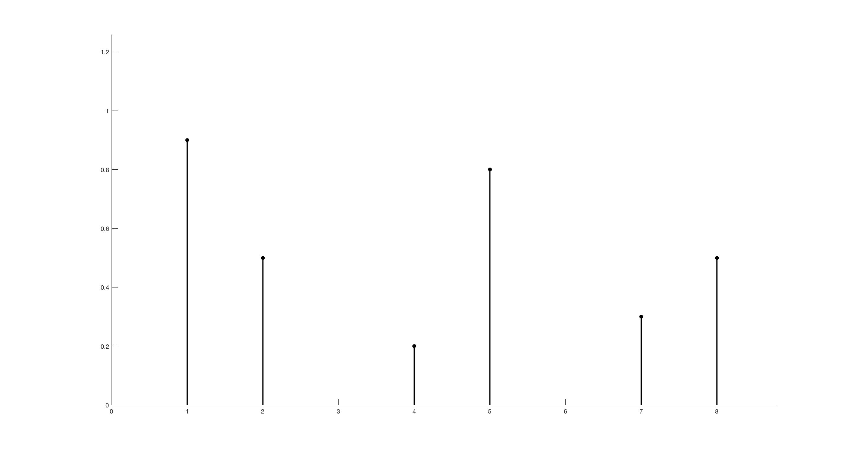
\[f(\mathbf{k})=\sum_{j=1}^{m}\delta(\mathbf{k}-\mathbf{k_j})q_j\]
\[\mathcal{F}(f(\mathbf{k}))=\int_{-\infty}^{\infty}\sum_{j=1}^{m}\delta(\mathbf{k}-\mathbf{k_j})q_je^{-2\pi i\mathbf{k}\mathbf{x}}d\mathbf{k}=\sum_{j=1}^{m}q_je^{-2\pi i\mathbf{k_j}\mathbf{x}}\]
Then
\[ \begin{align}\begin{aligned}(\text{sinc} \ast f)(\mathbf{a_i})=\int_{-\infty}^{\infty}\text{sinc}(\mathbf{a_i}-\mathbf{k})f(\mathbf{k})d\mathbf{k}\\=\sum_{j=1}^{m}q_j\int_{-\infty}^{\infty}\text{sinc}(\mathbf{a_i}-\mathbf{k})\delta(\mathbf{k}-\mathbf{k_j})d\mathbf{k}\\=\sum_{j=1}^m q_j\text{sinc}(\mathbf{a_i}-\mathbf{k_j})\end{aligned}\end{align} \]
Similarly
\[ \begin{align}\begin{aligned}(\text{sinc}^2 \ast f)(\mathbf{a_i})=\int_{-\infty}^{\infty}\text{sinc}^2(\mathbf{a_i}-\mathbf{k})f(\mathbf{k})d\mathbf{k}\\=\sum_{j=1}^{m}q_j\int_{-\infty}^{\infty}\text{sinc}^2(\mathbf{a_i}-\mathbf{k})\delta(\mathbf{k}-\mathbf{k_j})d\mathbf{k}\\=\sum_{j=1}^mq_j\text{sinc}^2(\mathbf{a_i}-\mathbf{k_j})\end{aligned}\end{align} \]
So, the desired quantities are \((\text{sinc} \ast f)(\mathbf{a_i})\) and \((\text{sinc}^2 \ast f)(\mathbf{a_i})\). But by the convolution theorem:
\[ \begin{align}\begin{aligned}(\text{sinc} \ast f)(\mathbf{a_i})=\mathcal{F}^{-1}(\mathcal{F}(\text{sinc})\mathcal{F}(f))(\mathbf{a_i})\\(\text{sinc}^2 \ast f)(\mathbf{a_i})=\mathcal{F}^{-1}(\mathcal{F}(\text{sinc}^2)\mathcal{F}(f))(\mathbf{a_i})\end{aligned}\end{align} \]
Luckily, \(\mathcal{F}(\text{sinc})\) and \(\mathcal{F}(\text{sinc}^2)\) take simple forms, which are derived below.
Fourier Transform of \(\text{Sinc}\)
1D
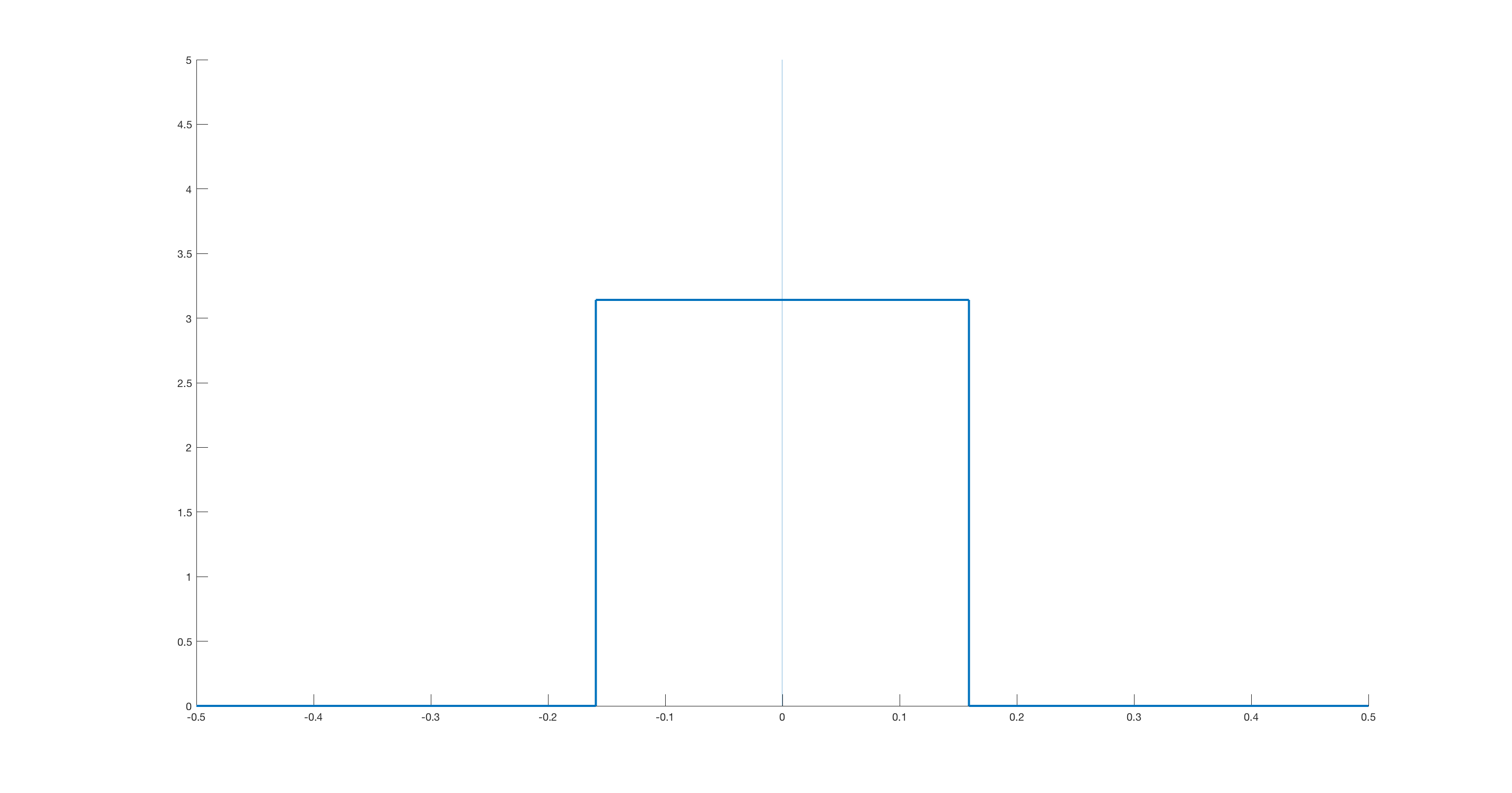
Consider the function
\[ \begin{align}\begin{aligned}h(x)= \: b \: \: \: \: |x|\leq a\\0 \: \: \: \: |x|>a\end{aligned}\end{align} \]
We have that
\[\mathcal{F}(h(x))(f)=\int_{-a}^{a}be^{-2\pi ixf}dx=2ab\text{sinc}(2\pi af)\]
Using the symmetry of Fourier transform, i.e. \(\mathcal{F}(h(x))(f)=h(-f)\), and that \(h(x)\) is even:
\[\mathcal{F}(H(x))(f)=\mathcal{F}(2ab\text{sinc}(2\pi ax))(f)=h(x)\]
Then \(h(x)\) with \(a=\frac{1}{2\pi}\) and \(b=\pi\) is equal to \(\mathcal{F}(\text{sinc}(x))(f)\), as shown below.
2D
Again, let
\[ \begin{align}\begin{aligned}h(x)= \: b \: \: \: \: x_1\leq a , \: x_2 \leq a\\0 \: \: \: \: x_1 > a , \: x_2 > a\end{aligned}\end{align} \]
\[\mathcal{F}(h(\mathbf{x}))(\mathbf{f})=\int_{-a}^{a}\int_{-a}^{a}be^{-2\pi i\mathbf{x}\mathbf{f}}d\mathbf{x}=4a^2b\text{sinc}(2\pi af_1)\text{sinc}(2\pi af_2)=4a^2b\text{sinc}(2\pi a\mathbf{f})\]
As before, setting \(a=\frac{1}{2\pi}\) and \(b=\pi^2\) yields \(\mathcal{F}(\text{sinc}(\mathbf{x}))(f)\)
3D
Let
\[ \begin{align}\begin{aligned}h(x)= \: b \: \: \: \: x_1\leq a , \: x_2 \leq a, \: x_3 \leq a\\0 \: \: \: \: x_1 > a , \: x_2 > a, \: x_3 > a\end{aligned}\end{align} \]
\[\mathcal{F}(h(\mathbf{x}))(\mathbf{f})=\int_{-a}^{a}\int_{-a}^{a}\int_{-a}^{a}be^{-2\pi i\mathbf{x}\mathbf{f}}d\mathbf{x}=8a^3b\text{sinc}(2\pi af_1)\text{sinc}(2\pi af_2)\text{sinc}(2\pi af_3)=8a^3b\text{sinc}(2\pi a\mathbf{f})\]
Setting \(a=\frac{1}{2\pi}\) and \(b=\pi^3\) yields \(\mathcal{F}(\text{sinc}(\mathbf{x}))(f)\)
Fourier Transform of \(\text{Sinc}^2\)
The following basic fact about convolution, combined with the previous section, will easily provide the Fourier transform of \(\text{sinc}^2\)
\[\mathcal{F}(\text{sinc}^2(\mathbf{x}))(\mathbf{f})=(\mathcal{F}(\text{sinc}(\mathbf{x})) \ast \mathcal{F}(\text{sinc}(\mathbf{x})))(\mathbf{f})\]
1D
\[ \begin{align}\begin{aligned}\mathcal{F}(\text{sinc}^2(\mathbf{x}))(\mathbf{f})= \pi(1-\pi|x|) \: \: \: \: |x|\leq \frac{1}{\pi}\\0 \: \: \: \: |x| > \frac{1}{\pi}\end{aligned}\end{align} \]
2D
\[ \begin{align}\begin{aligned}\mathcal{F}(\text{sinc}^2(\mathbf{x}))(\mathbf{f})= \pi^2(1-\pi|x_1|)(1-\pi|x_2|) \: \: \: \: |x_1|\leq \frac{1}{\pi}, \:|x_2|\leq \frac{1}{\pi}\\0 \: \: \: \: |x_1| > \frac{1}{\pi}, \:|x_2| > \frac{1}{\pi}\end{aligned}\end{align} \]
3D
\[ \begin{align}\begin{aligned}\mathcal{F}(\text{sinc}^2(\mathbf{x}))(\mathbf{f})= \pi^2(1-\pi|x_1|)(1-\pi|x_2|)(1-\pi|x_3|) \: \: \: \: |x_1|\leq \frac{1}{\pi}, \:|x_2|\leq \frac{1}{\pi}, \:|x_3|\leq \frac{1}{\pi}\\0 \: \: \: \: |x_1| > \frac{1}{\pi}, \: |x_2| > \frac{1}{\pi}, \: |x_3| > \frac{1}{\pi}\end{aligned}\end{align} \]
Implementation
Putting together the previous sections:
\[ \begin{align}\begin{aligned}(\text{sinc} \ast f)(\mathbf{k_i})=\mathcal{F}^{-1}(\mathcal{F}(\text{sinc})\mathcal{F}(f))(\mathbf{k_i})\\= \int_{\frac{-1}{2\pi}}^{\frac{1}{2\pi}}\pi\Big(\sum_{j=1}^{m}q_je^{-2\pi ik_jx}\Big)e^{2\pi ixk_i}dx\\= \frac{1}{2}\int_{-1}^{1}\Big(\sum_{j=1}^{m}q_je^{-ik_jy}\Big)e^{iyk_i}dy\end{aligned}\end{align} \]
In 2 and 3 dimensions, the constant \(\frac{1}{2}\) changes to \(\frac{1}{4}\) and \(\frac{1}{8}\), respectively, and integration is multidimensional with the same bounds.
\[ \begin{align}\begin{aligned}(\text{sinc}^2 \ast f)(\mathbf{k_i})=\mathcal{F}^{-1}(\mathcal{F}(\text{sinc}^2)\mathcal{F}(f))(\mathbf{k_i})\\=\int_{\frac{-1}{\pi}}^{\frac{1}{\pi}}\pi(1-\pi|x|)\Big(\sum_{j=1}^{m}q_je^{-2\pi ik_jx}\Big)e^{2\pi ixk_i}dx\\=\frac{1}{4}\int_{-2}^{2}(2-|y|)\Big(\sum_{j=1}^{m}q_je^{-ik_jy}\Big)e^{iyk_i}dy\end{aligned}\end{align} \]
Again, in 2 and 3 dimensions, the constant \(\frac{1}{4}\) changes to \(\frac{1}{8}\) and \(\frac{1}{16}\), respectively, and integration is multidimensional.
In each case, there are two main tasks: computing the inner summation, and computing the outer (possibly multidimensional) integral. But the inner summation is exactly a discrete (nonuniform) Fourier transform, and is computed with the finufft library. The outer integral again takes the form of of a Fourier transform (in the other direction), but since we want the exact integral, quadrature weights (either Gauss-Legendre of corrected trapezoidal, from Kapur-Rokhlin) are used to weight the integrand before again applying the finufft library. Note that in the case of \(\text{sinc}^2\), the integrand is only piecewise continuous, so the quadrature points are treated accordingly.